271,104 Routes: What I Missed About Mixture-of-Experts

This started while I was researching mixture-of-experts for a lab. I wanted to understand how a model could use only some of its parameters for each token and still perform well. Before getting into that, though, I needed to understand what an expert actually was.

I was also assuming that using fewer parameters meant needing less memory. That needs a bit more care: the experts that don't run for a token still have weights to store.

So I tried building the pieces in PyTorch. First I called a few toy experts, then added a router, then grouped the tokens into batches for those experts. Choosing the experts only took a few operations. Getting the rows into the right groups and returning the outputs was a larger part of the process than I'd expected.

After those examples, I ran code, math, prose, and multilingual prompts through IBM Granite and saved 271,104 routes. I wanted to see what a trained router selected, and whether the patterns changed between prompt groups.

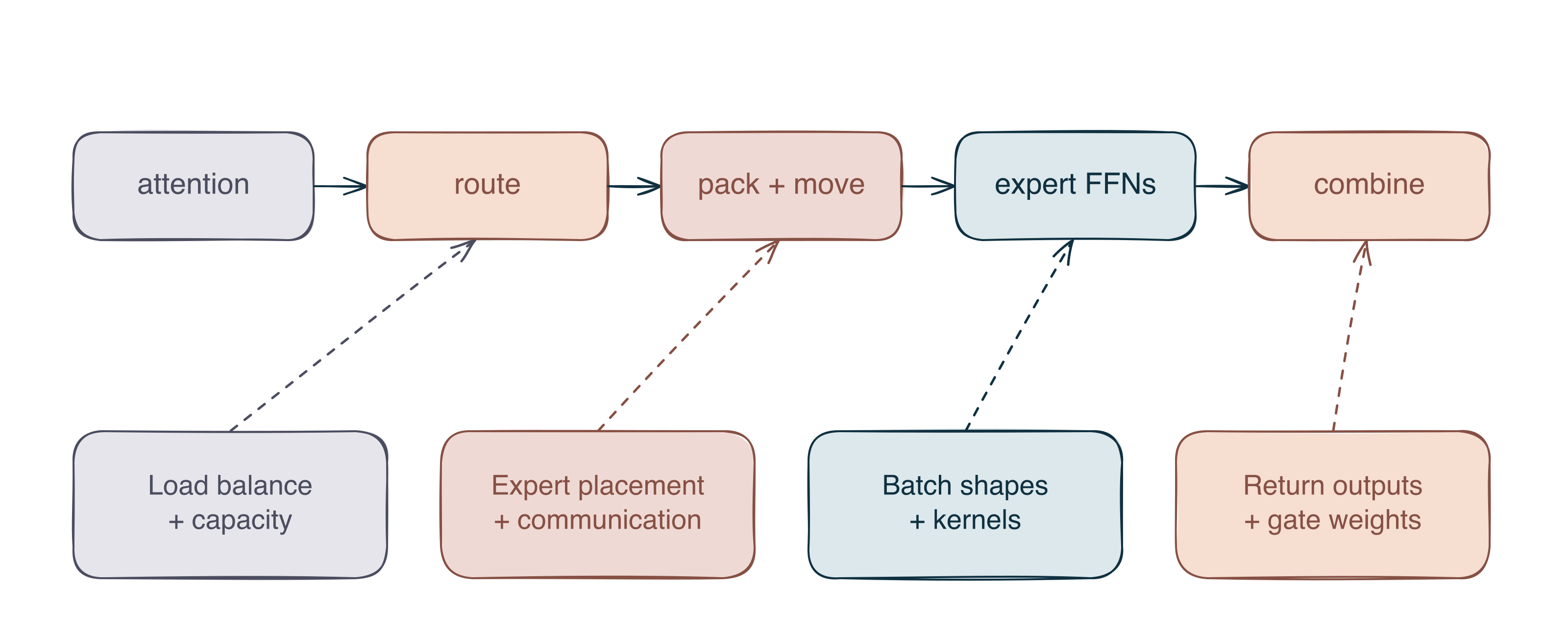
The path I'm following through the post is:

MoE layer = route + pack + move + compute + combine

I'm using Granite 3.1 1B-A400M. It has 24 MoE layers, with 32 routed experts in each layer, and each token gets eight of them. After excluding padding, my batch had 1,412 tokens. That's where the number in the title comes from:

1,412 tokens × 24 layers × 8 selected experts = 271,104 routes

1. What an expert actually is

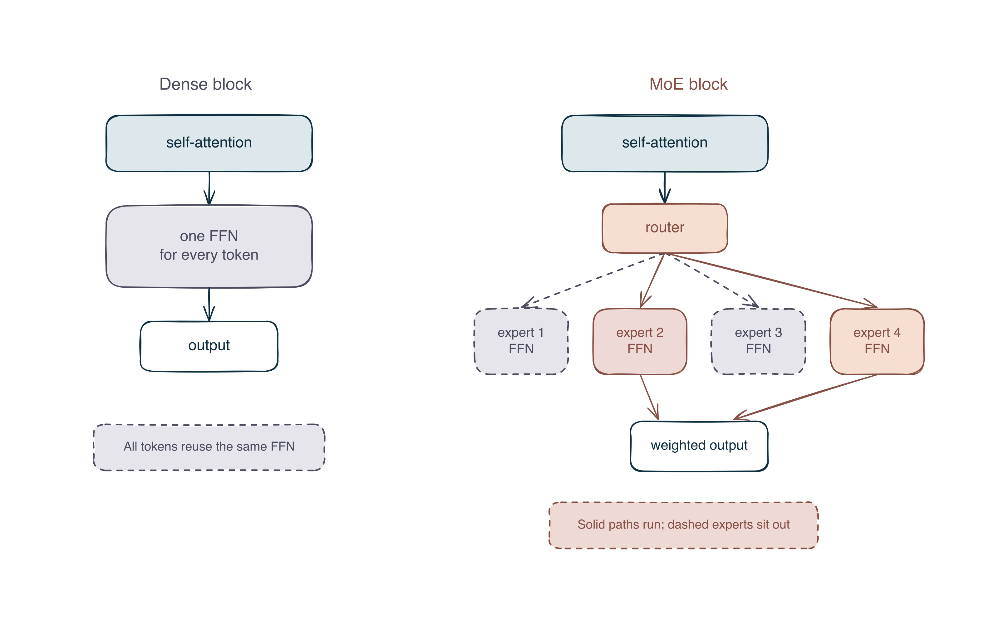
The name “expert” made me think of separate models for things like code and math. In the model I'm looking at here, an expert is a feed-forward network, or FFN, inside a transformer block. It takes a token's hidden state and transforms it.

There isn't a built-in label saying one expert handles math and another handles code. Whether they develop different functions is something I'd need to investigate.

Open full size ↗

Attention, normalization, and the residual connections are still there. Attention lets tokens exchange information across the sequence. In the feed-forward path, I now have several expert FFNs to choose from:

shared attention
    -> router
    -> selected expert FFNs
    -> combine
    -> shared residual path

An FFN processes each token row independently. That means I can collect the rows going to the same expert, run them together, and put the results back afterward. Attention is still responsible for mixing information between tokens. ^{1, 2, 3, 10}

For one token state x, I want a weighted sum of the selected experts' outputs:

y(x) = sum over selected experts i of p_i(x) * E_i(x)

Here, E_i(x) is expert i's output, and p_i(x) is the weight I give it.

I start with linear layers as toy experts and choose the expert IDs and weights myself. This lets me follow each call before adding a router. The loops add the weighted outputs into y, then I check the output shape and that the gate weights sum to one:

import torch

torch.manual_seed(0)
x = torch.randn(3, 4)
experts = [torch.nn.Linear(4, 4, bias=False) for _ in range(4)]
expert_ids = torch.tensor([[0, 2], [1, 2], [3, 0]])
gates = torch.tensor([[0.7, 0.3], [0.4, 0.6], [0.8, 0.2]])

y = torch.zeros_like(x)
for token in range(x.size(0)):
    for slot, expert_id in enumerate(expert_ids[token]):
        y[token] += gates[token, slot] * experts[expert_id](x[token])

assert y.shape == x.shape
assert torch.allclose(gates.sum(dim=-1), torch.ones(3))

With top-2 routing over 32 experts, a token goes through two expert FFNs. The other 30 don't run for that token. Each selected expert still does dense matrix multiplication; the saving comes from executing fewer of them.

The loops make this easy to follow, but they aren't how I'd want to run a large batch. Different tokens can choose different experts, and a GPU generally handles larger, regular matrix multiplications better than lots of tiny calls. I'll need to turn the individual choices into batches.

2. The router

The router chooses which experts to use. In this example, torch.nn.Linear maps each token's hidden state to one score, or logit, per expert. I take the two largest logits with topk(), then apply softmax over those two values to get the weights.

I'm also checking the shape of the selected IDs and that each token's weights sum to one:

import torch

torch.manual_seed(7)
tokens = torch.randn(4, 6)
hidden_size, num_experts, top_k = 6, 32, 2
router = torch.nn.Linear(hidden_size, num_experts, bias=False)
logits = router(tokens)
top_logits, expert_ids = logits.topk(k=top_k, dim=-1)
weights = top_logits.softmax(dim=-1)

assert expert_ids.shape == (len(tokens), top_k)
assert torch.allclose(weights.sum(dim=-1), torch.ones(4))

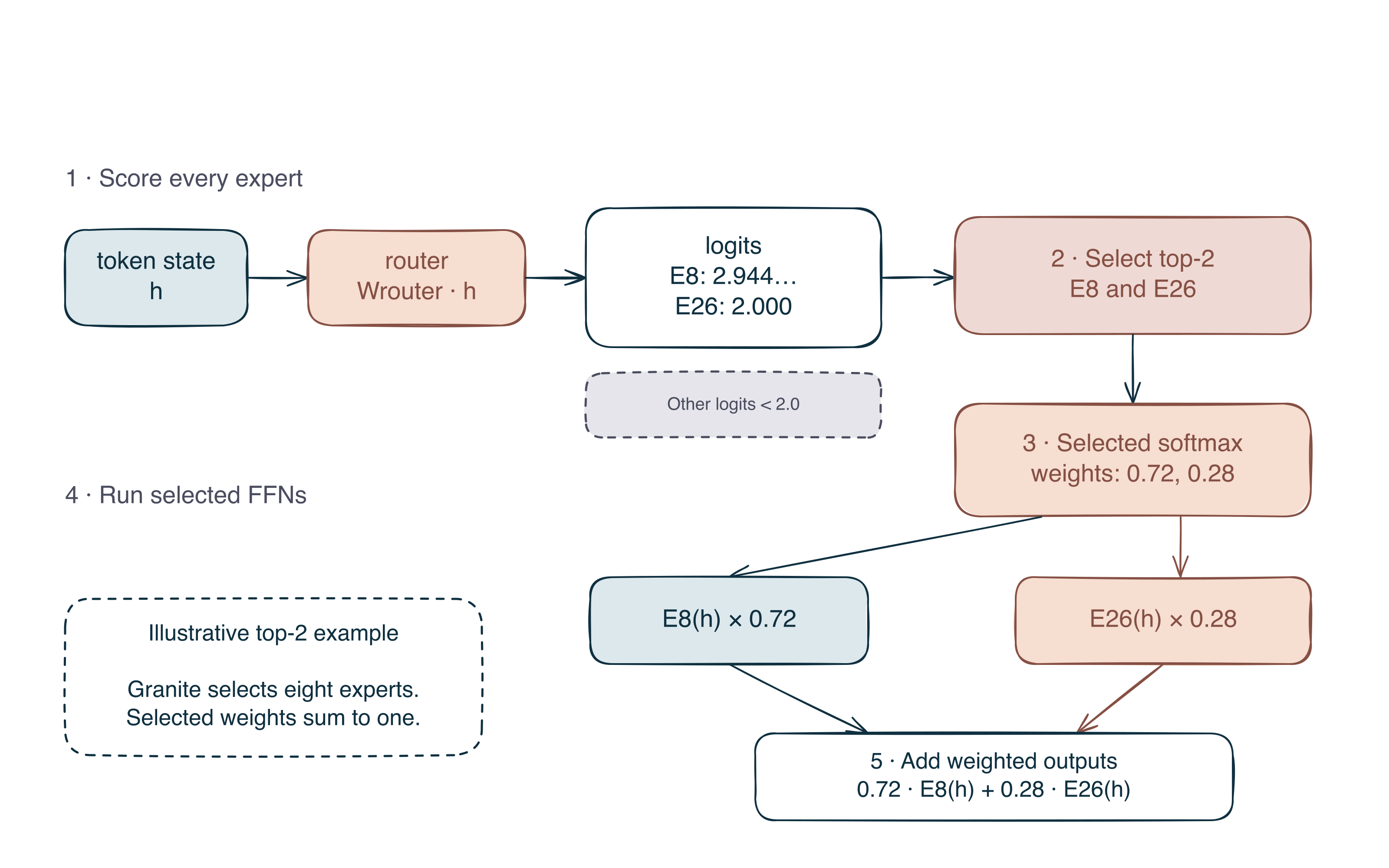
That gives me two outputs: expert_ids tells me which experts to call, and weights tells me how much of each output to use. For example:

expert_ids = [8, 26]
weights    = [0.72, 0.28]

For this token, I'd run experts 8 and 26, multiply their outputs by 0.72 and 0.28, and add them together. The weights sum to one. ^{1, 2, 3, 10}

Open full size ↗

The order of topk() and softmax matters here. Granite selects the top-k logits first and applies softmax to those selected values, so that's the order I'm using. Other implementations can calculate scores over the whole expert pool first. When comparing routers, I need to check the scoring and normalization to understand which weights reach the final sum. ^{3, 15, 16}

An expert ID only identifies a network within its layer. If expert 8 gets the highest weight here, that says something about this hidden state in this layer. Expert 8 in another layer is a different network, and the number alone doesn't tell me its function.

These choices also determine how many rows each expert processes, which experts receive examples during training, and potentially which device needs the rows. For T tokens with top-k routing, I create:

T * k token-expert assignments

That's the number of assignments before any capacity policy drops or changes routes. Granite selects eight experts, so each token creates eight assignments at every MoE layer. ^{15, 16}

At this point I have IDs and weights. The token activations are still where they started, so the next step is to gather the rows each expert needs.

3. Moving the tokens

I want to give each expert a batch containing the rows assigned to it. Since a token can go to more than one expert, its row can appear in more than one batch.

I'm keeping this example to three tokens so I can follow the assignments:

token 0 -> experts 2 and 7
token 1 -> experts 7 and 4
token 2 -> experts 2 and 4

Grouped by expert, those same assignments become:

expert 2 -> token 0, token 2
expert 4 -> token 1, token 2
expert 7 -> token 0, token 1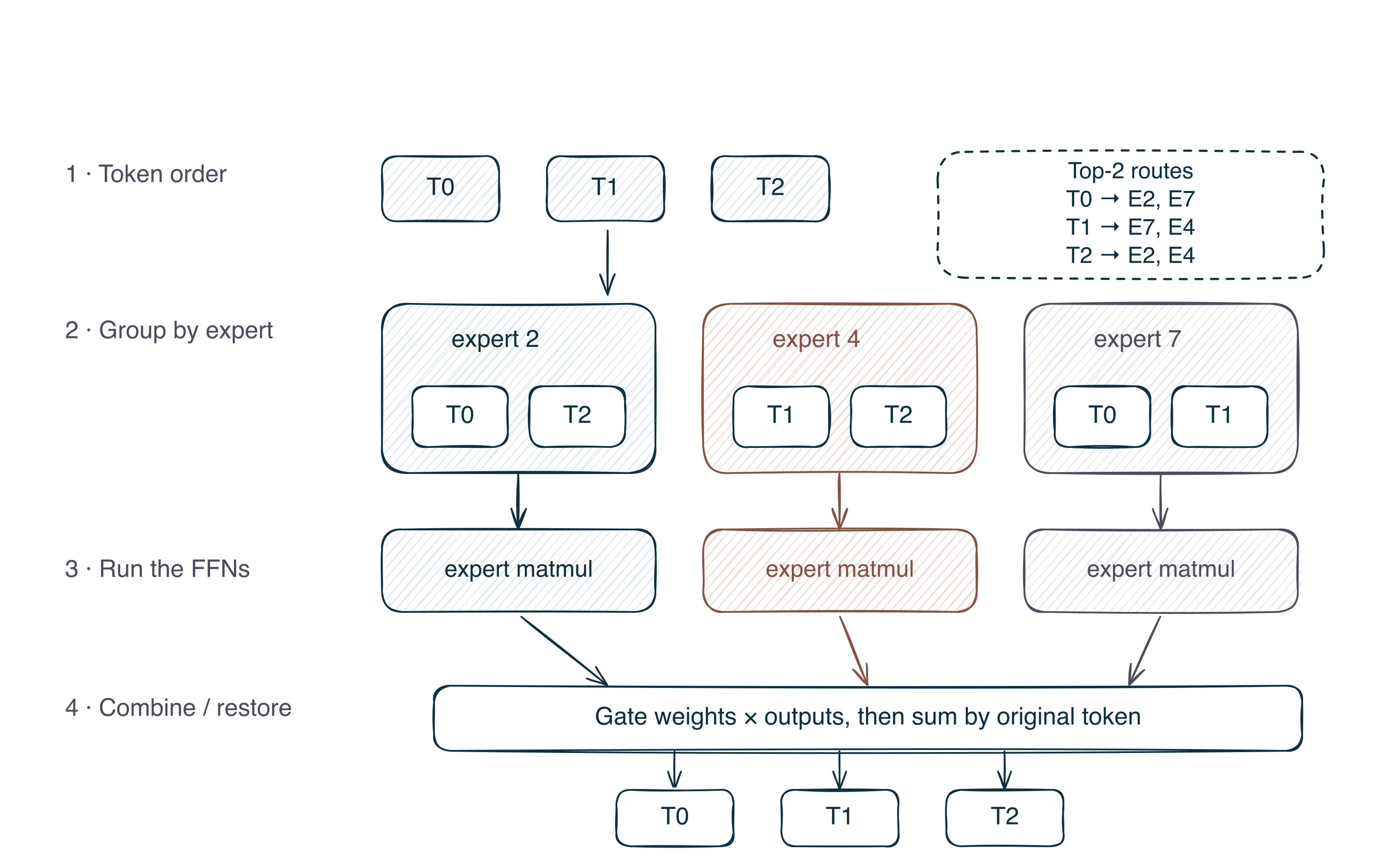

Open full size ↗

Each token now appears in two groups. To return the outputs correctly, the runtime needs to keep track of the original token, its selected expert, its position in the expert batch, and its gate weight. That information forms a route table.

This PyTorch example handles just the reordering. repeat_interleave gives me a token ID for each assignment, argsort groups the assignments by expert, and index_select gathers the rows.

Then restored[order] = packed puts each row back in its original assignment position. I check that against the original repeated rows and check the cumulative expert counts too. The FFNs and weighted combination aren't included in this example yet:

import torch

x = torch.tensor([[1.0, 1.1], [2.0, 2.1], [3.0, 3.1]])
expert_ids = torch.tensor([[2, 7], [7, 4], [2, 4]])
token_ids = torch.arange(len(x)).repeat_interleave(2)
flat_experts = expert_ids.flatten()
order = flat_experts.argsort(stable=True)
packed = x.index_select(0, token_ids[order])
expert_ends = torch.bincount(flat_experts, minlength=8).cumsum(0)

restored = torch.empty_like(packed)
restored[order] = packed
assert torch.equal(restored, x.index_select(0, token_ids))
assert expert_ends.tolist() == [0, 0, 2, 2, 4, 4, 4, 6]

Including the expert computation gives me this sequence:

token-order activations
    -> duplicate rows for top-k routes
    -> sort or group by expert
    -> move rows to the expert owner
    -> run expert FFNs
    -> move outputs back
    -> undo the grouping
    -> apply gate weights and add
    -> original token order

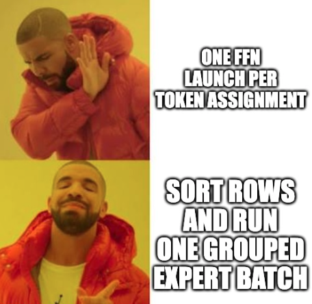
For Granite, there are eight assignments per token at each layer. Calling an FFN separately for every assignment would give me the right arithmetic, but it would also create a lot of small GPU launches.

Open full size ↗

Packing gathers an expert's rows into a batch so its matrix multiplication has more work to do at once. When I say the router sends a token to an expert, this is part of what needs to happen: the runtime uses the routing information to index, move, and batch the rows.

Too many tokens, same expert

The batches don't have to be the same size. One expert might get 40 assignments while another gets three.

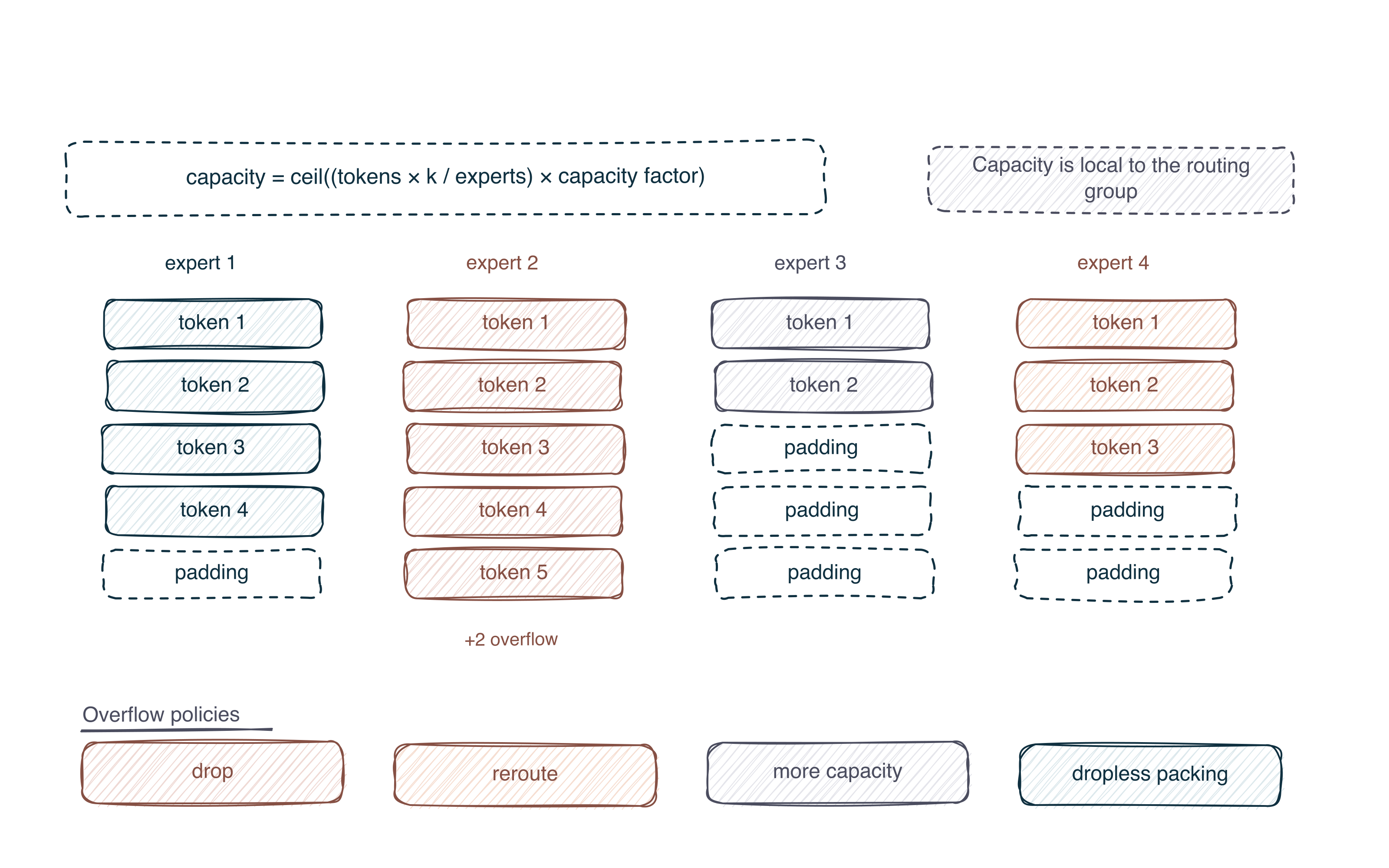
Some implementations reserve a fixed number of slots for each expert to keep tensor shapes predictable. That limit is the expert capacity. If too many assignments go to one expert, it can run out of slots even while another expert has room left.

Open full size ↗

There are a few ways to handle the extra assignments. Dropping routes changes the computation the router selected. Rerouting changes where they go. Reserving more capacity gives the busy expert more room, but can leave unused padding elsewhere. Dynamic packing can keep the routes, provided the metadata and kernels support variable loads. ^{3, 7}

During training, an expert that keeps getting selected also gets more examples to learn from. That can reinforce the router's preference while other experts receive fewer examples. During synchronous execution, the busiest expert or device can also keep the rest waiting.

Open full size ↗

I'd want to look at both the load distribution and model quality. Equal traffic doesn't prove the assignments are useful, and uneven traffic can still come with good language-model loss. ^{3, 4}

Putting them on different GPUs

The examples so far group rows locally. If the selected expert lives on another GPU, the token's activations need to travel to that device. After the expert runs, its output needs to come back to the device that owns the token.

That's why a typical expert-parallel layer has two communication steps:

source token owners
    -> dispatch all-to-all
    -> local expert computation
    -> combine all-to-all
    -> source token owners

The first all-to-all sends rows to the devices holding the selected experts. Each participating process, or rank, can have rows for several other ranks, and the amounts can differ. The second all-to-all returns the expert outputs to the original token owners. Then I can combine them and continue through the transformer.

To understand the cost, I'd need to measure more than the total bytes transferred. Message sizes, the number of peers, network layout, packing overhead, and the slowest rank all matter. The routing choices determine where the traffic goes; the runtime and cluster determine how that traffic gets handled. ^{2, 8, 9}

4. Trying Granite

The small examples let me follow the operations. Next I wanted to see what a trained router would do with actual text.

I'm using the Granite 3.1 1B-A400M base checkpoint, with 24 MoE layers, 32 routed experts per layer, and top-8 routing. I put together 48 fixed prompts: 12 each for code, math, prose, and multilingual text. Each prompt gets its own batch element, truncated at 96 tokens.

After excluding padding, that leaves 1,412 tokens: 493 code, 266 math, 260 prose, and 393 multilingual. The groups have the same number of prompts, but different numbers of tokens. That matters when interpreting the counts.

I ran an inference-only forward pass and saved the selected experts and their weights, giving me 271,104 assignments. This measures routing on the supplied text. It doesn't involve training, text generation, or a serving-speed benchmark. ^{15, 16}

This is the part of the code that extracts the choices and weights:

with torch.inference_mode():
    output = model(
        **batch,
        output_router_logits=True,
        use_cache=False,
    )

for router_logits in output.router_logits:
    top_logits, expert_ids = router_logits.float().topk(8, dim=-1)
    weights = top_logits.softmax(dim=-1)

Since Granite applies softmax over the eight selected logits, each token's weights should sum to one. I check that before interpreting the results:

gate_sums = weights.sum(dim=-1)
torch.testing.assert_close(
    gate_sums,
    torch.ones_like(gate_sums),
    atol=1e-6,
    rtol=0,
)

The largest error was 2.38e-7. I also reran fixed prompts from each domain to check that the extraction was consistent. The selected expert IDs matched exactly, and the largest weight difference was zero. ¹⁶

Open full size ↗

What showed up

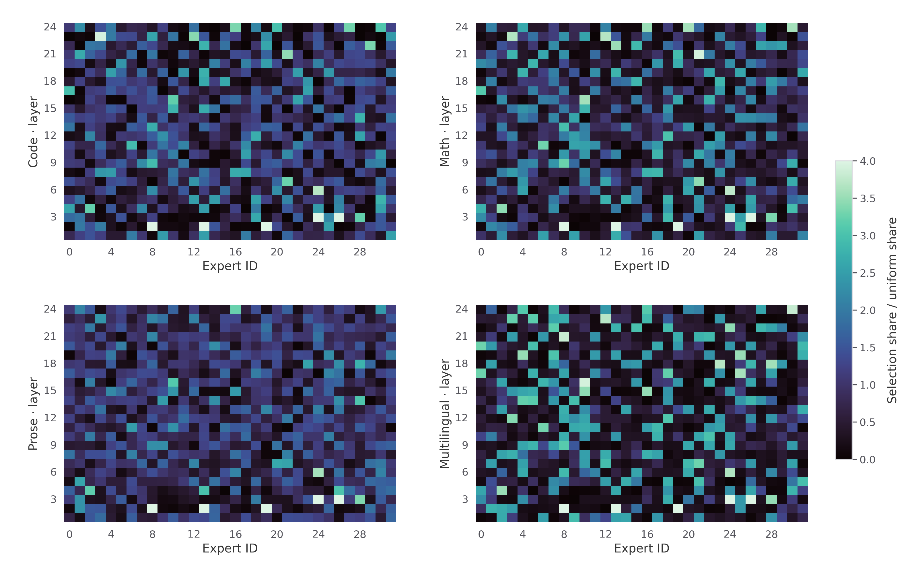
In the aggregated selection counts, expert 8 had the largest share for code, math, and multilingual tokens. Expert 26 led for prose. Those leading shares were around 4% to 5%. A perfectly uniform distribution across 32 experts would give each one 3.125%.

That doesn't give me enough evidence to call expert 8 a coding expert. I'm adding up counts for layer-local IDs, and expert 8 across 24 layers isn't one shared module. What I can say is that this ID was selected more often for code in this sample.

The gate weights give me another way to look at the routes. Selection counts tell me how often an expert is used, but the selected outputs can receive very different weights.

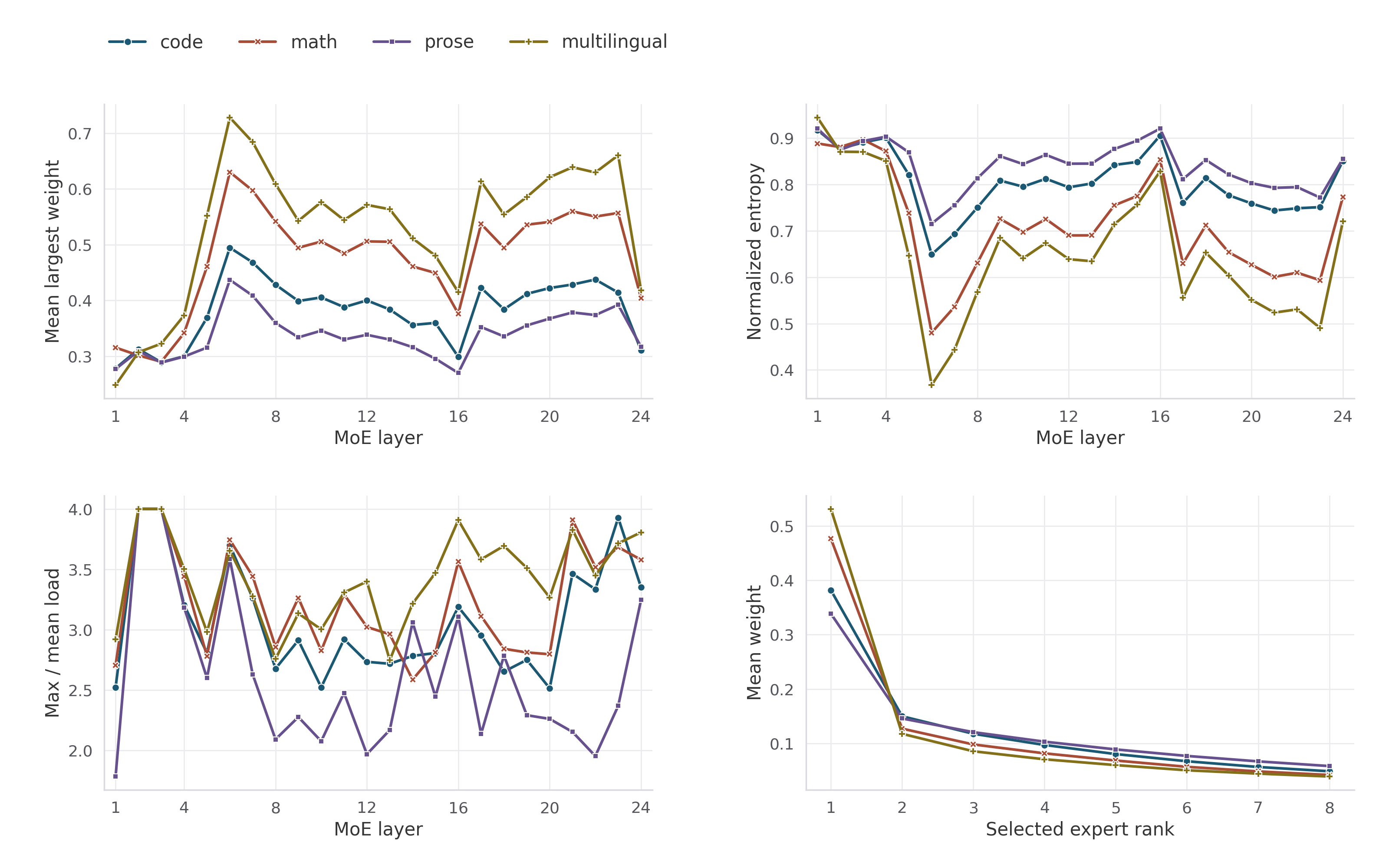
Averaged across layers, the largest selected weight was 53.1% for multilingual tokens and 33.9% for prose. Normalized routing entropy, which describes how spread out the selected weights are, was 65.7% for multilingual and 84.2% for prose. Multilingual tokens tended to concentrate more weight on one of their eight experts, while prose spread the weights more evenly. That's why I'm keeping both the selection counts and the gate weights.

Code and math had the most similar expert-load patterns. Their mean layer-wise Jensen–Shannon distance was 0.169, while code and multilingual were farthest apart at 0.287. Lower means more similar here. This compares where the traffic went; it doesn't establish what the experts understand.

Looking at layers individually, I found that in layers 2 and 3, one expert appeared in every sampled token's top eight within each domain. Its load was four times the average. That's also the maximum possible ratio for this setup: one expert can receive T assignments, while the average is 8T / 32.

Later layers showed different patterns across domains. An overall average would hide those differences, so I kept the layer-by-layer plots too.

If you're comparing these numbers with the saved files, I'm numbering layers 1–24 to match the experiment and plots. Expert IDs are zero-based.

Open full size ↗

What this doesn't tell me

This is one checkpoint and a small hand-built prompt set, with different token counts between groups. The percentages describe this sample. I'd want to check other workloads before expecting the same patterns elsewhere.

I also haven't established what each expert computed or whether it caused a particular output. Selection counts and gate weights only take me so far. Testing specialization would need something like ablations, expert swaps, output comparisons, or feature-level analysis. I haven't run those experiments here.

5. Where I ended up

The small PyTorch examples gave me a way to check each step. I could follow an assignment into an expert batch, restore its position, and compare the tensor with what I expected.

The router's choice affects the whole layer. Different tokens run through different FFNs, and during training only the selected experts receive that token's expert-path gradients. ^{1, 3, 4} The assignments also set the batch sizes and, when experts are on different devices, where activations need to travel.

MoE layer = route + pack + move + compute + combine

Coming back to my memory question, the full expert pool still needs to be stored somewhere. I can split it across devices or fetch weights when needed. Selecting fewer experts reduces the expert arithmetic for a token, but it doesn't remove the other weights or settle where they should live. ^{10, 13}

The effect on speed depends on how the model runs. With tiny expert batches, launch overhead and weight movement can dominate. With large expert-parallel groups, communication can take a lot of the time. Given enough rows per expert, the matrix multiplications can become the main cost. The route counts alone don't tell me which of those is limiting a run. ^{7, 8, 9, 13}

For another MoE implementation, I'd start by checking the number of assignments and how they're batched. Then I'd look at which experts get many rows or almost none, which routes cross devices, and how large those messages are. If the traffic changes between domains, I'd also want to separate that observation from any claim about what the experts do.

There are more directions to explore, including alternate routers, upcycling, parallelism layouts, specialized kernels, and serving. For this post, I kept the focus on following the token path and inspecting the Granite routes.

What I'd try next

I'd like to profile serving with different batch sizes and expert-parallel layouts next. In one trace, I'd want the router counts, packing, first all-to-all, expert matrix multiplications, second all-to-all, combine, and per-expert load. That would let me compare the time spent at each step with the routing choices and device layout.

I haven't run that yet. For now, I've got a way to follow the token assignments and some measured differences between the prompt groups. That's enough to give me a more specific question for the next experiment: where does the time actually go?

Thanks for reading :)