ROGII Wellbore Geology Prediction

by Michael Rusu

I combined particle filtering, pretrained tree ensembles, and per-well calibration to estimate where a horizontal well sits within the rock layers. The engineering challenge was keeping the ensemble manageable in memory while preserving its numerical precision.

Competition

ROGII Wellbore Geology Prediction
Kaggle · Calibrated ensemble V50

Explore the project ↓

The problem

A horizontal well can travel through different geological layers even when its physical depth changes very little. I worked on predicting True Vertical Thickness (TVT), the well’s position within that geological sequence, in feet.

The inputs are the well trajectory, its gamma-ray log, the already interpreted prefix, and a reference typewell with a vertical gamma-ray signature. The task is to align those signals and continue the geological interpretation into the portion where TVT is hidden. The competition data description defines the inputs and prediction zone.

The geological cross-section above is schematic. Its layers and path explain the task; they are not measured well data or model predictions.

My contribution

I adapted public alignment recipes and pretrained model artifacts into the V50 ensemble. My work focused on how the branches fit together: residual mixing, stratigraphic projection, calibration against each well’s visible prefix, and the memory behavior of the complete inference path.

The pretrained trees come from Ravaghi’s and Fleongg’s public artifacts. The recipe also builds on public notebook implementations and Pilkwang Kim’s stratigraphic-alignment work. I credit those sources below; the underlying pretrained models are upstream contributions.

Architecture

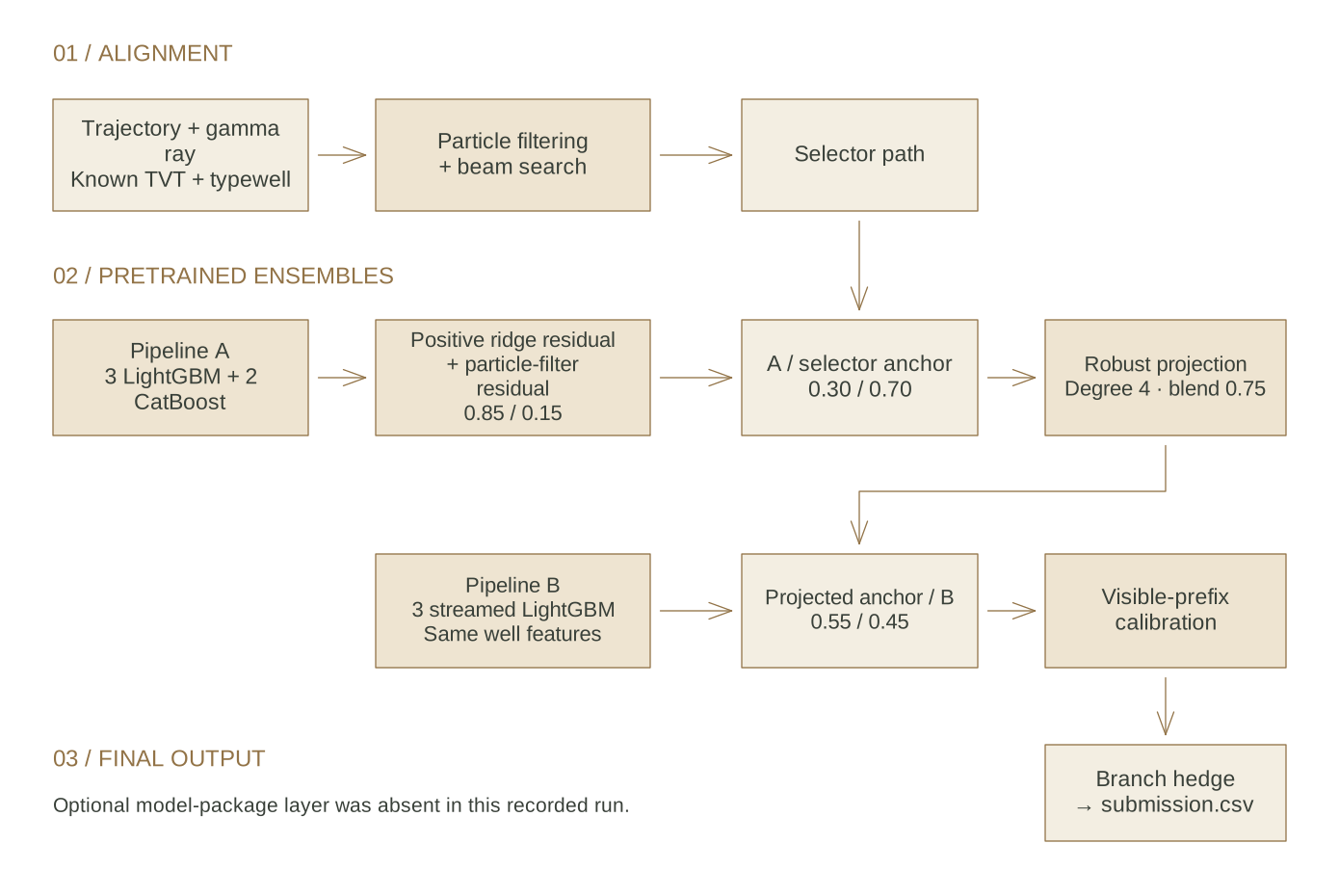
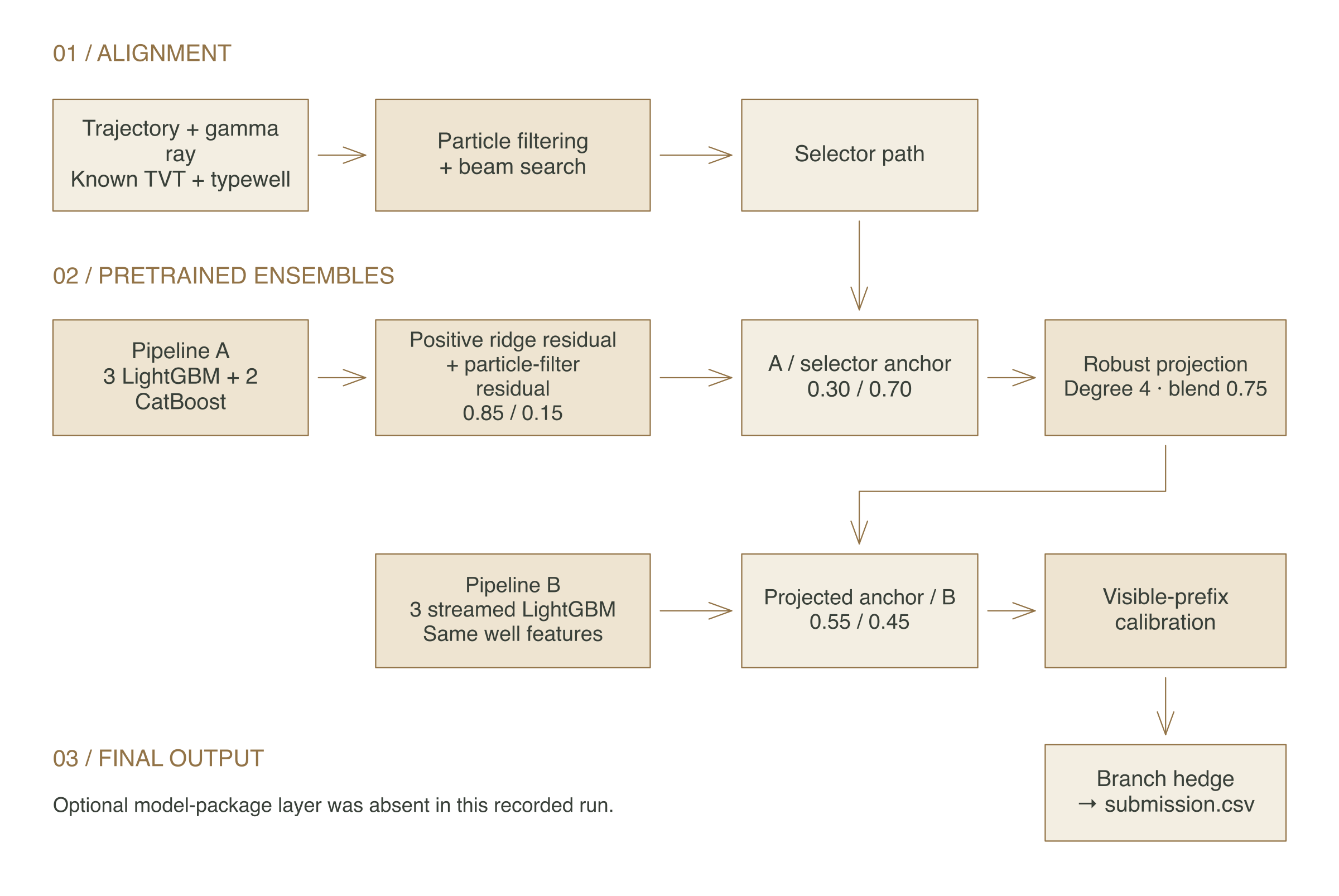
Figure 1. Two learned branches and a physical alignment path feed the calibrated ensemble. PNG Editable Excalidraw Download figure

I start with particle-filter and beam-search paths that compare the horizontal gamma-ray log with the typewell. A selector supplies an alignment anchor. Pipeline A then combines three LightGBM trainers and two CatBoost trainers through a positive ridge stack built from their saved out-of-fold predictions.

The ridge residual and particle-filter residual use weights of 0.85 and 0.15, with an exponential warm-up over 85 units of measured depth. I mix that branch with the selector at 0.30 / 0.70, apply a robust degree-four stratigraphic projection at a 0.75 blend, and combine the projected anchor with Pipeline B’s three streamed LightGBM models at 0.55 / 0.45.

Python · Residual warm-upV50 · lines 1675–1681

warmup = 1.0 - np.exp(
    -np.maximum(test_df["md_since"].to_numpy(dtype=float), 0.0) / residual_tau
)
d = residual_alpha * warmup * (
    (1.0 - pf_residual_weight) * ridge_test + pf_residual_weight * pf_delta
)
pred = last + d

An excerpt from the retained V50 source: the warm-up controls how strongly residual predictions move away from the last known TVT.

Calibration

Each well has a known prefix that I can use for local checks. I mask the end of that prefix at 50%, 65%, and 75% cut points, compare candidate continuations with the known values, and use their error and consistency to select a calibration path.

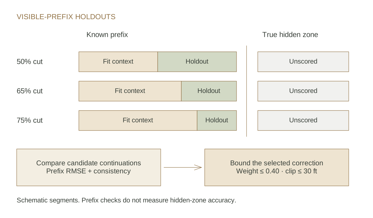
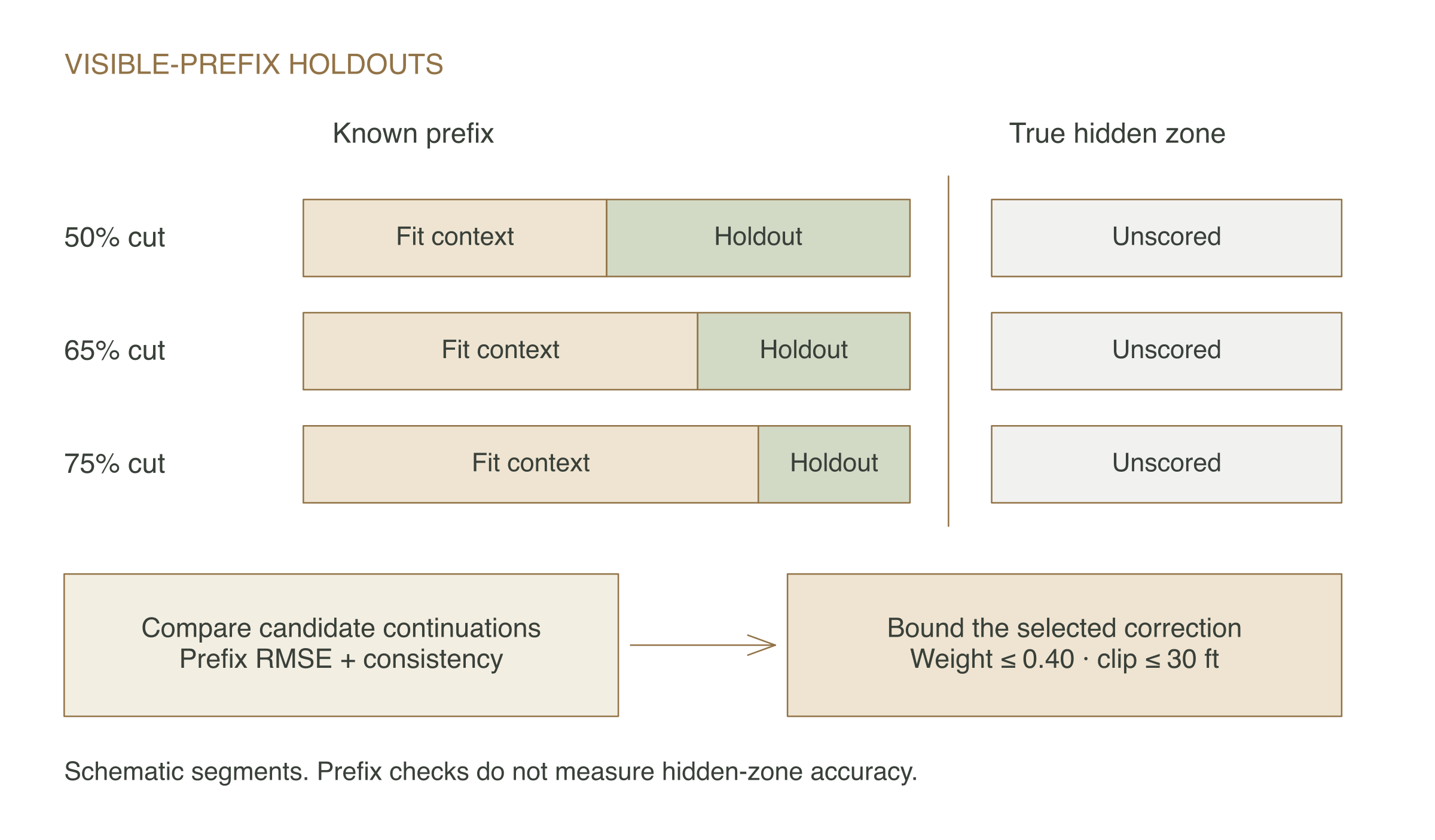
Figure 2. I test continuations within the visible prefix before adjusting the hidden-zone prediction. Segment lengths are schematic. PNG Editable Excalidraw Download figure

The balanced profile limits the calibration weight to 0.40 and its correction clip to 30 feet. This keeps a locally promising candidate from replacing the entire ensemble. A final particle-filter branch hedge can make a small correction when the seed runs support a second path; it applied to one of the three example wells.

The source also supports an optional manifest-driven frontier model package. That package was absent in the retained run, so its layer left the prefix-calibrated base unchanged before the final branch hedge.

Memory management

The feature table was described in my notebook as over 7 GB. I avoided loading it in full: Pipeline A reads the header for feature order, runs each serialized trainer in an isolated subprocess, and retains compact prediction arrays. Pipeline B loads one model at a time.

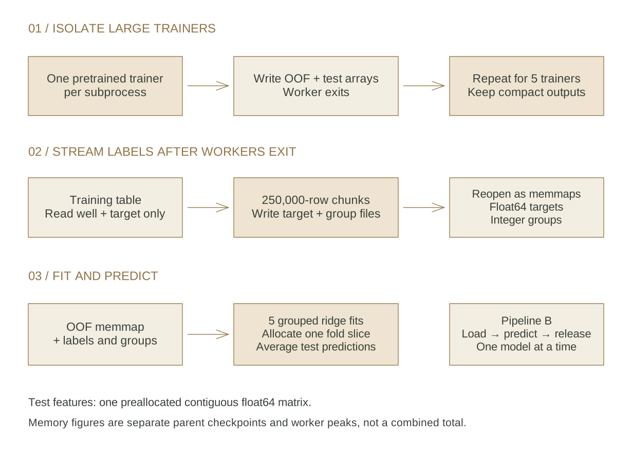
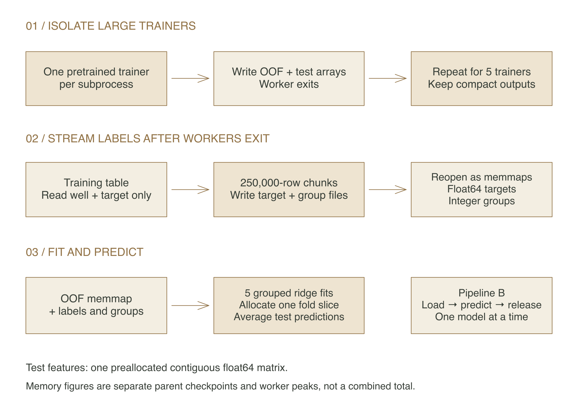
Each isolated trainer writes predictions and exits. Only the well and target columns stream in 250,000-row chunks into disk-backed arrays. Five ridge fits use these arrays; Pipeline B loads its three models one at a time. — Figure 3. Large objects have bounded lifetimes, while labels, groups, and out-of-fold predictions stay on disk. PNG Editable Excalidraw Download figure

I fill test features directly into one contiguous float64 array. Targets and well groups stream in 250,000-row chunks into files that I reopen as NumPy memmaps, avoiding a full Python list and concatenation step. The ridge fits still allocate their training-fold slices; disk-backed storage does not remove every in-memory allocation.

Python · Disk-backed labels and groupsV50 · lines 1397–1404

y = np.memmap(target_path, mode="r", dtype=np.float64, shape=(total,))
groups = np.memmap(group_path, mode="r", dtype=group_dtype, shape=(total,))
print(
    f"Pipeline A labels complete: {len(y):,} rows, {len(group_names)} wells, "
    f"groups={np.dtype(group_dtype).name}, storage=disk-backed",
    flush=True,
)
return y, groups

The final lines of the label-streaming function reopen the completed arrays without loading them in full.

I kept pandas because the serialized estimators and feature builders already expect that interface. Feature matrices, out-of-fold predictions, targets, and ridge fitting remain float64; the well-group codes use compact integers. The tradeoff is additional disk I/O and subprocess startup time.

Evaluation and results

The competition evaluates TVT predictions using RMSE. My retained V50 output documents an example inference run, not an evaluation on the hidden competition wells. Kaggle replaces the visible example wells when it reruns a submitted notebook.

Recorded measurement	V50 example run
Prediction rows	14,151 across 3 example wells
Streamed training labels	3,783,989 rows across 773 wells
Runtime	Approximately 501 seconds
Largest parent RSS checkpoint	0.697 GiB
Largest isolated-worker peak RSS	0.769 GiB
Submission audit	14,151 rows; id, tvt columns; ID order matches the sample

The parent measurement is the largest recorded checkpoint, and the worker measurement is the largest reported peak from an isolated trainer. Neither is the combined process-tree memory peak. These numbers describe this example run and do not establish full hidden-test runtime or memory usage.

The ridge stage uses five well-grouped fits and averages their test predictions. The visible-prefix holdouts guide calibration, but the retained output does not provide an independent, end-to-end accuracy result. I’m reporting the completed run and its submission checks without claiming a leaderboard improvement.

The final audit checks the two-column submission, sample ID order, and prediction hashes. One submission-shaped file remains: submission.csv. The next useful evaluation is a held-out-well comparison of the complete ensemble and its calibration branches, alongside a measurement of total process-tree memory.

Competition and references

I used the V50 source and its saved console output for the implementation details, excerpts, and measurements on this page. The public artifacts and recipe references are linked below.

Open the ROGII competition